The magnetic field of the Large Magellanic Cloud
Mapping the field of our nearest gas-rich galaxy from polarized dust and from the motions of its atomic hydrogen, and picking out its cold neutral phase.
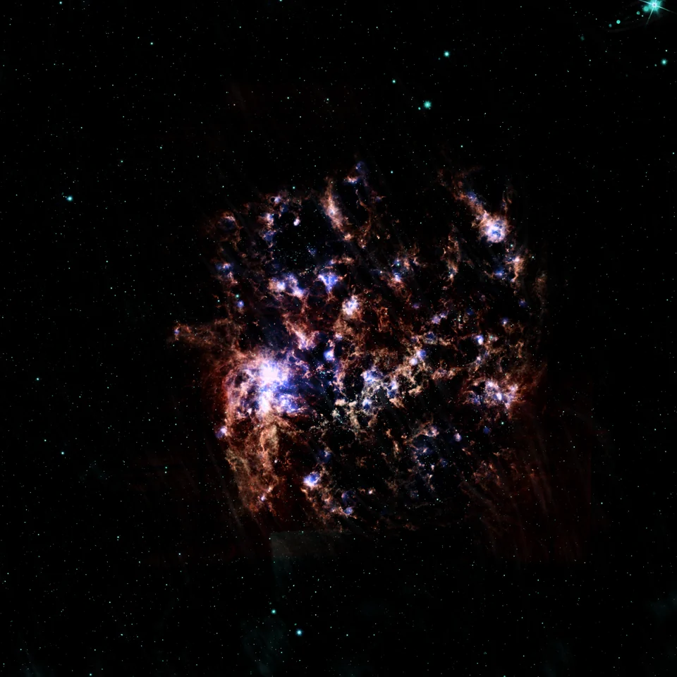
The LMC is 162 000 light years away and inclined by only 25 to 35 degrees, so its whole disk fits in one map. Planck measured the polarized emission of its dust at 353 GHz. Rotated by 90 degrees, the polarization angle gives the plane-of-sky orientation of the magnetic field, but the map also contains the polarized dust of the Milky Way in front of the LMC.
Alina et al. (2023) removed that foreground. Its polarization direction came from velocity gradients in GASS H I and was checked against starlight polarization; its intensity came from the dust-to-gas correlation around the galaxy. After the subtraction the field follows the atomic gas, notably along the molecular ridges south and south-east of 30 Doradus and along the southern arm that extends towards the Small Magellanic Cloud. The maps on this site show Planck before that correction.
The foreground direction comes from the velocity gradient technique. It assumes that turbulent motions stretch the structures seen in thin velocity channels of 21 cm data along the magnetic field, so the gradients run perpendicular to it. In the published LMC work it gave the direction of the Milky Way foreground, not the field of the LMC itself. The premise is debated: some studies read the striations in channel maps as cold density filaments. Hu, Lazarian, Alina et al. (2023) argued from simulated multiphase H I and GALFA-HI data that thin channels are dominated by velocity fluctuations, so the striations trace the turbulent velocity field and align with the field best in the thinnest channels.
The same 21 cm spectra also separate the cold neutral medium from the rest of the atomic gas. Molecular clouds form out of the cold phase.
Results
What the papers report, in their own terms. Each item links to its source.
With the Milky Way foreground removed, the plane-of-sky field of the LMC tends to follow its atomic gas, notably along the molecular ridges south and south-east of 30 Doradus and along the southern arm that extends towards the Small Magellanic Cloud.
Alina et al. 2023The median polarization fraction of the LMC after foreground removal is slightly lower than in the diffuse Milky Way, and the distribution as a whole is similar.
median p = 3.6% (4.0% before removal; 5.3% for the Milky Way, Planck Int. XIX)
Alina et al. 2023The highest polarization fractions in the LMC, a conservative lower limit on the maximum, are close to those measured for the Milky Way.
pmax = 21.6% (99th percentile; Milky Way 19.8% and 22%)
Alina et al. 2023In simulated multiphase H I and in GALFA-HI data, thin velocity channels are dominated by the velocity contribution: the striations aligned with the field are mainly velocity caustics, and the alignment is strongest in the thinnest channels.
Hu et al. 2023
Look through the layers
Every layer below is public survey data on one 12° grid. Choose a base map and a lens layer.
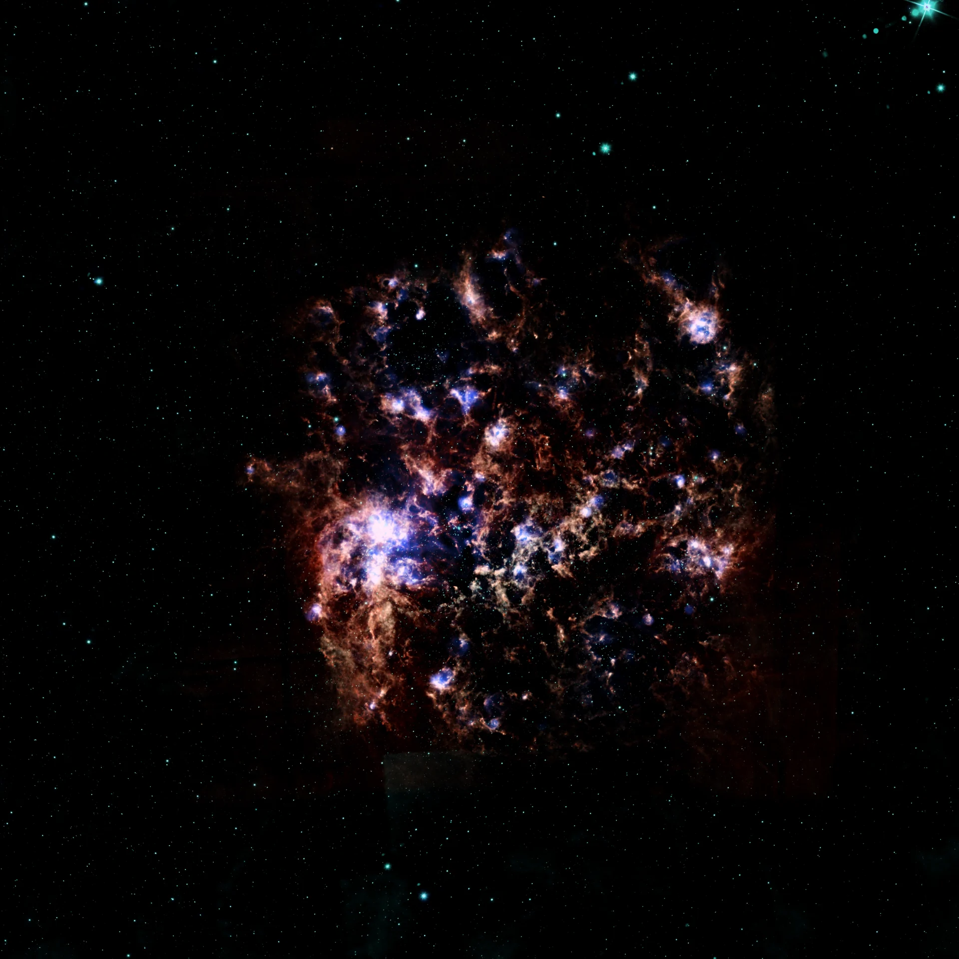
Multi-band composite
- Data
- SHASSA H-alpha, beam 48″ (0.8' resolution, 48'' pixels) · Gaustad et al. 2001WISE 12 µm, beam 6.5″ · Wright et al. 2010Herschel SPIRE 250 µm, beam 18″ · Griffin et al. 2010WISE 3.4 µm, beam 6.1″ · Wright et al. 2010
- Stretch
- Per band: background removal, asinh stretch from a percentile black point, starlet sharpening, colour screen blend (scripts/composites.py).
- Scale
- LMC, width 12.1° at 49.59 ± 0.09 (stat) ± 0.54 (sys) kpc (Pietrzynski et al. 2019)
- Script
- scripts/composites.py composite(), scripts at e462b02-dirty
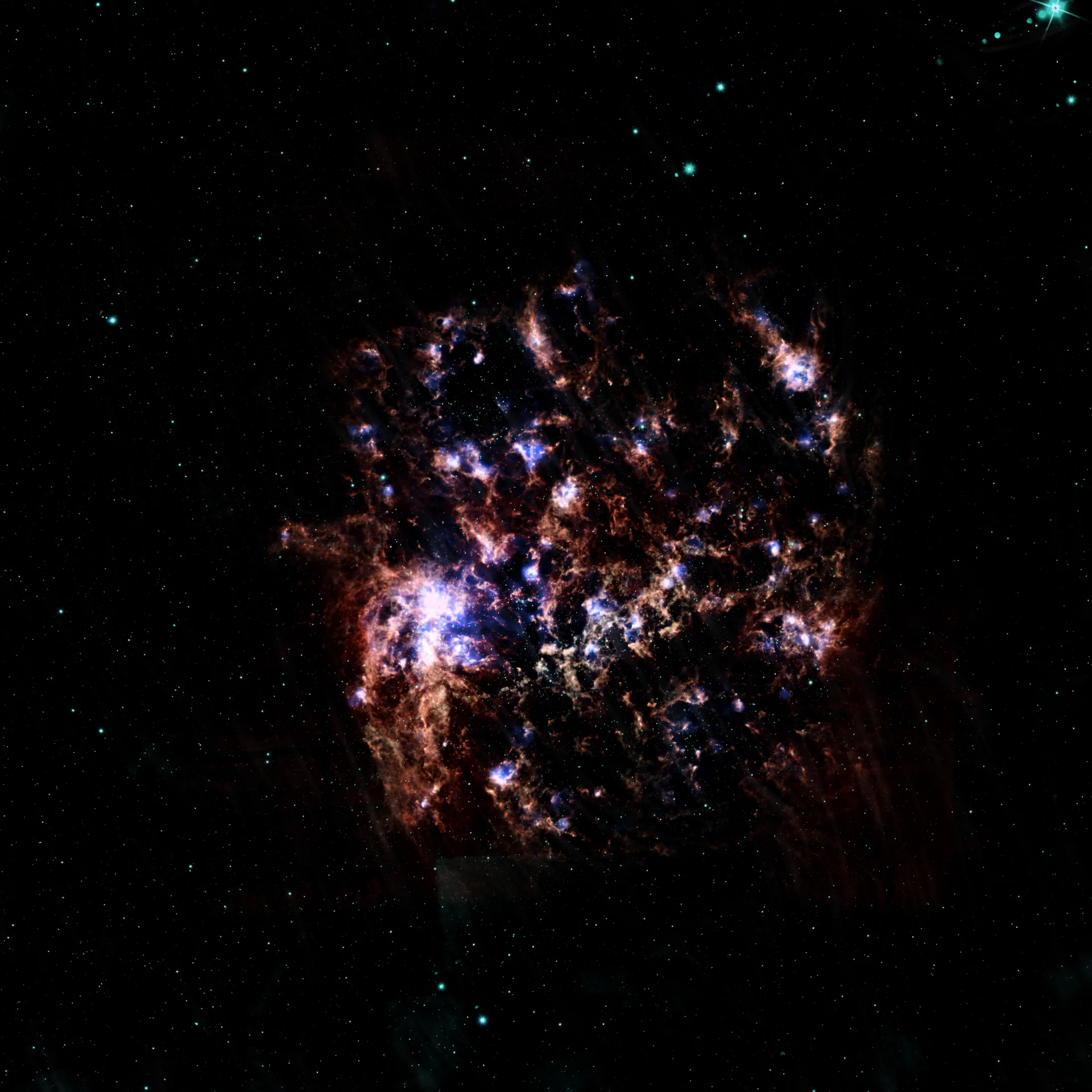
Composite with the Planck field
- Data
- SHASSA H-alpha, beam 48″ (0.8' resolution, 48'' pixels) · Gaustad et al. 2001WISE 12 µm, beam 6.5″ · Wright et al. 2010Herschel SPIRE 250 µm, beam 18″ · Griffin et al. 2010WISE 3.4 µm, beam 6.1″ · Wright et al. 2010Planck 353 GHz (PR4), beam 4.9′ (effective beam FWHM 4.94') · Planck Collaboration III 2020
- Stretch
- Per band: background removal, asinh stretch from a percentile black point, starlet sharpening, colour screen blend (scripts/composites.py).
- Smoothing
- Field texture: Q and U smoothed with a 10′ sigma Gaussian (FWHM 24′ with the Planck beam), then drawn as line integral convolution.
- Polarized S/N
- Above 3 over 89% of the field (median 12.4). Noise from the PR4 covariances, white between pixels; a lower bound.
- Scale
- LMC, width 12.1° at 49.59 ± 0.09 (stat) ± 0.54 (sys) kpc (Pietrzynski et al. 2019)
- Script
- scripts/composites.py composite(), scripts at e462b02-dirty
- Download
- lmc_field_angle.fits 1.2 MB · Field position angle, east of north (deg)lmc_field_snr.fits 1.2 MB · Polarized S/N at the field smoothingCredits and licence are in the FITS header.
Ridge filter, Herschel 250 µm
- Data
- Herschel SPIRE 250 µm, beam 18″ · Griffin et al. 2010
- Stretch
- Strongest negative Hessian eigenvalue of log intensity at sigma 1.5, 3 and 6 pixels (scale-normalised), normalised to the 99.5th percentile.
- Scale
- LMC, width 12.1° at 49.59 ± 0.09 (stat) ± 0.54 (sys) kpc (Pietrzynski et al. 2019)
- Script
- scripts/composites.py ridges(), scripts at e462b02-dirty
Planck dust with the field texture
- Data
- Planck 353 GHz (PR4), beam 4.9′ (effective beam FWHM 4.94') · Planck Collaboration III 2020
- Stretch
- Dust stretch as the intensity image; the line integral convolution texture is added to the value before the colour map (amount 0.4).
- Smoothing
- Q and U smoothed with a 12 pixel (8′) Gaussian, FWHM 20′ with the beam. Angle drawn in grid coordinates (render_lmc.grid_angle).
- Polarized S/N
- Above 3 over 87% of the field (median 9.95). Noise from the PR4 covariances, white between pixels; a lower bound.
- Scale
- LMC, width 12.1° at 49.59 ± 0.09 (stat) ± 0.54 (sys) kpc (Pietrzynski et al. 2019)
- Script
- scripts/render_lmc.py planck_maps(), lic(), scripts at e462b02-dirty
- Download
- lmc_field_angle.fits 1.2 MB · Field position angle, east of north (deg)lmc_field_snr.fits 1.2 MB · Polarized S/N at the field smoothingCredits and licence are in the FITS header.
Planck 353 GHz intensity
- Data
- Planck 353 GHz (PR4), beam 4.9′ (effective beam FWHM 4.94') · Planck Collaboration III 2020
- Stretch
- asinh (softening 0.2) between the 2nd and 99.8th percentile (0.745 to 16.413 mK_CMB), copper palette.
- Smoothing
- Unsmoothed; the solar dipole is fitted away from the plane and removed.
- Scale
- LMC, width 12.1° at 49.59 ± 0.09 (stat) ± 0.54 (sys) kpc (Pietrzynski et al. 2019)
- Script
- scripts/render_lmc.py read_planck(), render main(), scripts at e462b02-dirty
- Download
- lmc_planck353_I.fits 1.2 MB · Planck 353 GHz intensity (K_CMB)Credits and licence are in the FITS header.
H I column density
- Data
- GASS H I, beam 16′ (gridded; the Parkes beam is 14.3') · McClure-Griffiths et al. 2009
- Stretch
- Moment 0 over 182 to 339 km/s (LSR), asinh (softening 0.15) between the 2nd and 99.9th percentile (0 to 2753 K km/s), grey palette. Column density assumes optically thin gas, 1.823e+18 cm⁻² per K km/s.
- Smoothing
- Cube reprojected to the 40″ grid (bicubic).
- Scale
- LMC, width 12.1° at 49.59 ± 0.09 (stat) ± 0.54 (sys) kpc (Pietrzynski et al. 2019)
- Script
- scripts/render_lmc.py hi_products(), scripts at e462b02-dirty
H I mean velocity
- Data
- GASS H I, beam 16′ (gridded; the Parkes beam is 14.3') · McClure-Griffiths et al. 2009
- Stretch
- Intensity-weighted mean velocity from 200 (blue) to 320 km/s (red), RdBu_r; brightness is the H I column to the power 0.8. Pixels below the 35th percentile of the column are set to the median velocity.
- Smoothing
- Cube reprojected to the 40″ grid (bicubic).
- Scale
- LMC, width 12.1° at 49.59 ± 0.09 (stat) ± 0.54 (sys) kpc (Pietrzynski et al. 2019)
- Script
- scripts/render_lmc.py hi_products(), scripts at e462b02-dirty
CO(1-0) clouds
- Data
- MAGMA CO(1-0), Mopra, beam 45″ (33'' beam, gridded to about 45'') · Wong et al. 2011
- Stretch
- Moment 0 of channels above 3 sigma (MAGMA rms cube), asinh (softening 0.1) between the 5th and 99.8th percentile (0.4 to 27.6 K km/s); drawn as cyan with opacity from the stretch.
- Smoothing
- Reprojected to the 40″ grid.
- Scale
- LMC, width 12.1° at 49.59 ± 0.09 (stat) ± 0.54 (sys) kpc (Pietrzynski et al. 2019)
- Script
- scripts/render_lmc.py co_moment0(), scripts at e462b02-dirty
Polarized signal to noise
- Data
- Planck 353 GHz (PR4), beam 4.9′ (effective beam FWHM 4.94') · Planck Collaboration III 2020
- Stretch
- Linear grey from 0 to 20; the red line marks S/N = 3.
- Smoothing
- Same smoothing as the field texture (8′ sigma). S/N above 3 over 87% of the grid and 98% within 4° of the centre.
- Polarized S/N
- Above 3 over 87% of the field (median 9.95). Noise from the PR4 covariances, white between pixels; a lower bound.
- Scale
- LMC, width 12.1° at 49.59 ± 0.09 (stat) ± 0.54 (sys) kpc (Pietrzynski et al. 2019)
- Script
- scripts/map_meta.py smoothed_snr(), scripts at e462b02-dirty
- Download
- lmc_field_snr.fits 1.2 MB · Polarized S/N at the field smoothingCredits and licence are in the FITS header.
The composite with the Planck 353 GHz field orientation woven in. Move over the map; the lens shows a second layer.
H I under the pointer
Move over the map to see the 21 cm spectrum there. Drag on the spectrum to choose a velocity window. Move the red cut to see the rotation of the disc.
N(H I), cm⁻²
- RA, Dec
- move over the map
- l, b
- -
- Tb peak
- -
- N(H I), window
- -
GASS III H I (Parkes, 16′ beam; McClure-Griffiths et al. 2009, Kalberla and Haud 2015), LSR radio velocities, resampled to 0.08° pixels on the 12° field. The cube begins at 182 km/s, so Milky Way gas near 0 km/s is not in it. The spectrum axis shows only what is there; above 340 km/s the channels hold noise and are dropped, and at 182 km/s the cube cuts into Magellanic Bridge gas. N(H I) = 1.823×10¹⁸ ∫Tb dv assumes optically thin 21 cm emission; dense gas is underestimated. Masses use 49.59 kpc (Pietrzyński et al. 2019) and hydrogen only. The cut starts along the line of nodes, Θ = 139° (van der Marel and Kallivayalil 2014), through the H I dynamical centre (Kim et al. 1998). Colour scale follows the window.
Resolution and noise
The field drawn live from Planck Q and U. Smoothing more lowers the noise and blurs the structure; streaks fade where the polarized signal is weak.
In progress
Results appear here once they are published.
Field from GASKAP-HI velocity gradients
The same velocity-gradient method applied to GASKAP-HI 21 cm data, at 30 arcsecond resolution instead of the 16 arcminutes of GASS.
Cold neutral medium, separated
Gaussian decomposition of every H I spectrum (ROHSA) separates the cold neutral medium from the rest of the atomic gas.
Papers
4 entries from NASA ADS. All publications →
- 2026Magnetic field structure of the LMC: Insights from Atomic gas data and foreground emission separationAlina, Bernard, Yuen et al.IAU Symposium, 20, 179
- 2024The Magnetic Field Structure of the Large Magellanic Cloud: Insights from Atomic Gas Data and Foreground Emission SeparationAlina, Bernard, Yuen et al.32nd General Assembly International Union (IAUGA 2024), 103
- 2023Unveiling polarized emission from interstellar dust of the Large Magellanic Cloud with PlanckAlina, Bernard, Yuen et al.Monthly Notices of the Royal Astronomical Society, 518, 4466 · arXiv:2205.012756 cit.
- 2023Nature of striation in 21 cm channel Maps: velocity causticsHu, Lazarian, Alina et al.Monthly Notices of the Royal Astronomical Society, 524, 2994 · arXiv:2306.1000520 cit.